A D 7 5 1 v 2 0 0 8 . 0 2 . 1 2
D O C U M E N T A T I O N
Install
License
Analysis settings
Reading the windows
Handling the data files
Version history
AD751’s name explained
Windows XP standalone version
Image samples are to be found in the batch directory.
- Double-click on MCRInstaller_***.exe to install the Matlab Component Runtime.
- Unzip ad751_***w.zip and double-click ad751.exe to launch AD751.
Matlab version
- Download the AD751 file compatible with your Matlab version
- Unzip the .zip file
- Copy the ave folder under the Matlab directory toolbox
- Start Matlab and add the toolbox/ave/ path with subfolders to the Matlab search path ( [ File > Set path > Add with Subfolders ] )
- Start AD751 from the Matlab command by typing ad751
Functions from the following toolboxes are used: image processing, mapping, neural network, satistics.
Image samples are to be found in the batch directory.
based on the MIT Open Source License:
http://www.opensource.org/licenses/mit-license.htmlCopyright (c) 2002- Vlad ATANASIU & Multimedia Press - AD751
Permission is hereby granted, free of charge, to any person obtaining a copy of this software and associated documentation files (the "Software"), to deal in the Software without restriction, including without limitation the rights to use, copy, modify, merge, publish, distribute, sublicense, and/or sell copies of the Software, and to permit persons to whom the Software is furnished to do so, subject to the following conditions:
The above copyright notice and this permission notice shall be included in all copies or substantial portions of the Software.
THE SOFTWARE IS PROVIDED "AS IS", WITHOUT WARRANTY OF ANY KIND, EXPRESS OR IMPLIED, INCLUDING BUT NOT LIMITED TO THE WARRANTIES OF MERCHANTABILITY, FITNESS FOR A PARTICULAR PURPOSE AND NONINFRINGEMENT. IN NO EVENT SHALL THE AUTHORS OR COPYRIGHT HOLDERS BE LIABLE FOR ANY CLAIM, DAMAGES OR OTHER LIABILITY, WHETHER IN AN ACTION OF CONTRACT, TORT OR OTHERWISE, ARISING FROM, OUT OF OR IN CONNECTION WITH THE SOFTWARE OR THE USE OR OTHER DEALINGS IN THE SOFTWARE.
Figure 1.
The settings window (see legend in Reading the windows)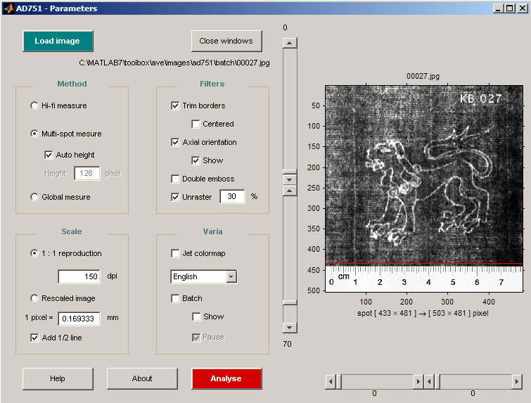
Figure 2. - below
Rotating the image (see legend in Reading the windows)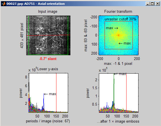
Figure 3. - below
Measuring the spot densities and computing global statistics (see legend in Reading the windows)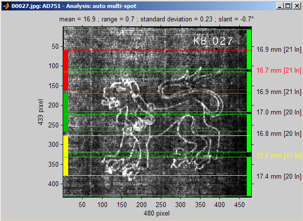
Button – [ Load image ]
- Buttons
Load image
Close windows
Help
About
Analyse- Methods
Hi-fi measure
Multi-spot measure
Global measure- Filters
Trim borders
Centered
Axial orientation
Double emboss
Unraster- Scale
1:1 reproductions
Rescaled image
Add ½ line- Varia
Jet colormap
Language
Batch / Show / PauseThis button opens a file explorer dialog box, letting you chose the image(s) you want to analyse. It will be displayed on the right side of the windows and its path under the [ Load image ] button. Its dimensions are given beneath it.
Supported image formats are jpg, tif (compressed tif's are not supported and such files will be skipped), bmp, png, pcx, hdf, xwd.
It is possible to analyse images one by one or in batches. In the later case you can load an image from the folder wich contain all the images you want to analyse, check the [ Batch ] checkbox and press the [ Analyse ] button. Files that cannot be processed are skept.
You can also write a txt file containing the absolute adresses of the image files - thus it is possible to process images in different directories and subdirectories in just one batch. Example:
C:\\MATLAB6p5\toolbox\ave\images\ad751\batch\00027.jpg
C:\\MATLAB6p5\toolbox\ave\images\ad751\batch\00027.jpg
...A listing of the files in a directory can be obtained by creating in the specified directory a text file dir.txt, opening and writing dir /a:-d /b /o:n /s >"files.txt" in it, then and changing its name to dir.bat. Double-clicking on dir.bat runs a DOS programe that writes the directory's content to the file files.txt.
Sample images are provided in the batch directory. Don't forget to make copies if you intend to empty the directory. A ready-made dir.bat file is supplied with AD751.
Closes all windows opened during the analysis process.
Opens this file in a web browser.
Author, version and acknowledgements for AD751.
Once all settings were chosen, pressing this button will start the image analysis. All data are automatically saved in files at the location where the image or batch file is located.
This is the most precise method, but also the most slow one. It looks over the whole image for spots of exactly 20 even spaced laid lines, computing their respective densities. Spots with aberrant values are discarded (a difference greater than 1mm from the values given by a auto multi-spot measurement). If no 20 lines spot is found, the multi-spot measure will be used.
All density measurements are made by considering the distance between the middle of the 1st laid line to one pixel before the middle of the 20st line. The formula is:
laid lines density in mm = (20 + ½ [if the option 'Add 1/2 line' is seletced]) * scale [mm for 1 pixel] * ( spot height in pixels / lines per spot )In publications allways document that densities are given in millimeters over 20 laid lines (plus ½ line if option selected).
Method – [ Multi-spot measure ]
This method moves a spot of fixed width at a specified interval across the whole image and computers the spot density. The density that would be that of 20 lines is inferred from the actual spot density, whatever the number of laid lines in it. This is the source of a slight difference from the hi-fi mode.
AD751 attempts to have spot heights with 20 lines. Therefore the height of the spot is deduced by dividing the entire image height by the total number of lines and multiplied by 20. The step of the spot movement is half its height.
To maximise the analysis sensibility the spots are equal in width to the image.
Aberrant values are disregarded. Is considered ‘aberrant’ a spot not containing between 16 & 24 lines.
It is possible to skip from automatic height evaluation to manual height setting. This feature can help fine-tune a particular spot so that it contains exactly 20 lines.
In the global method the density is given by the number of laid lines covering the space between the first line in the image to one pixel before the last one.
Blurs in the image can cause one or more lines to disappear – this is a supplementary reason to why the global measure is less precise than the hi-fi measure.
By using the sliders by the side of the image you can chose for analysis just one region of interest out of the whole image. It is however strongly recommended that borders such as rules superposed on the image, be cut off.
You cannot trim an image if there is no image loaded - as is the case when you start AD751. Load an image in order to trim it.
This option allows you to define a region of interest centered on the center of the image. It's dimension will not vary if the image is replaced (unless the subsequent image is smaller, in which case the region is reduced to the image's dimension).
The option is usefull if you want to analyse a group of images of varying dimensions and want to keep the dimension of the analysed region constant. It also helps eliminate borders on different sized images.
If this option is unchecked, AD751 will cut a constant number of pixels counting from the outside inwards.
Please note that in this case and if you batch images where you start with a large sized image and trim a surface bigger than the total surface of any following image, the trim will be reset to zero to accomodate the change in size.
Filters – [ Axial orientation ]
In order to give correct results the laid lines have to be horizontal. By enabling this checkbox the image will be axially orientated and you can see the slant analysis by enabling show.
In the case of strongly compressed images, such as low quality jpg files, you have to uncheck this box, otherwise the results will be erroneous.
In some type of images there are regularities much stronger than that of the laid lines. One example is the typographical raster in the case of paper structure reproductions scanned from books. Another example are rubbings made on thin paper where the imprint of the woven band of the industrialy made paper is visible. For such cases the unraster option will suppress most interferencies. The preset cutoff value supresses 30% of the highest frequencies. You can modify this value.
(If you don't get good results, look at the 'Fourier transform' in the NW of the 'Axial orientation' window: if there are many maximas (red dots) inside the red square increase the cutoff value until they fall outside the square).
Scale – [ 1 : 1 reproduction ]
In order to compute the density, AD751 has to know the real life dimensions of the supplied image. In the case you use reproduction methods such as electronradiography or betagraphy, the resulting image will be in a 1:1 proportion to the original paper. To how many millimetres corresponds a pixel will depend on the scanning resolution. For image in a 1:1 scale digitised at 150 dpi, 1 pixel is 0.169333… mm.
The formula is : 25.4 / [scanning resolution in dots-per-inch (dpi)].
If your image reproduce a paper at another scale than 1:1, you have to enable this setting and give the value of 1 pixel expressed in millimetres.
In the last twenty years of the 20th century the measurement of laid lines density as the length in millimeters covered by 20 ½ consecutive lines emerged as a standard practice (this is the unit used by default by AD751). More lines would have been difficult to count manually without mistakes (especially on low quality reproductions) and fewer lines yield too much variation across the paper. The additional half line helps avoid the problem of finding the exact position just before the middle of the last counted laid line, a maximum grey tonality probably being easier to detect by a human eye than the value just below it. Standard laid lines measurements are done on 20 ½ lines. If you have good reasons to use a density expressed for just 20 lines, then you can uncheck this option.
In publications allways document that densities are given in millimeters over 20 laid lines (plus ½ line if option selected).
Changes the color appearence of grayscale previsualization images. Can be usefull to emphasize aspects of the image, such as the attachement points of watermarks to the screen.
The information displayed on windows or saved in files can be in Dutch, English, French, German or Italian.
Varia – [ Batch / Show / Pause ]
If you check this option all the images in the current directory will be analysed. They can be displayed and a pause made in-between so that you can inspect the analysis (press a key on the keyboard to move on to the next image - the images are left open on the screen for further examination and comparison). To spare time you can uncheck these last two options – a percentage bar will show you then the progress of the analysis.
You can cancel the batch process at any time without loosing the information from the images allready analysed: data is saved as soon as an image was analysed.
The parameters window contains the command buttons described above, the analysis settings and a display of the image to be analyses.
The axial orientation is the second window that will show up in the case you enabled the appropriate option. The NW corner image shows the image to be analysed, after trimming and the slant (red line) found after orthogonalisation. For the axial orientation just a square in the middle of the image will be used (circumscribed by a green line). The Fourier transform is performed on this region (NE corner, displayed is the power spectrum) and the frequency corresponding to the laid lines indicated by arrows. Sideviews of the Fft facilitate the visualisation of its magnitudes on the FFTs of both the unfiltered and filtered image. If 'unraster' is enabled, then the cutoff frequency is displayed.
The laid lines frequency corresponds to the maximum on the Y-axis starting after the last frequency considered as noise. This threshold was found by filtering the image with a 90° ‘emboss’ filter, which would cut the low frequencies and leave as maximum magnitude of the Fft the laid lines frequency. Then the threshold will be set 4 units (if double emboss is unchecked, 15 units) lower than the maximum and the real lines frequency computed on the non-filtered input image.
The analysis window displays the location of the different analysed spots, with their respective densities and – for the multi-spot and global method – the number of lines they contain. The maximum density spot is displayed in red and those with aberrant values in yellow. Finally statistical measurements are provided:
- spot mean density for 20 ½ lines (or 20 according to the user’s settings);
- range of variation (maximum – minimum spot density);
- standard deviation (of the sample, not population);
- slant of laid lines before axial orientation.
Both spot and statistical data are saved in files.By clicking with the right mouse button on the image or on the window itself, the image can be magnified. By holding down the mouse and moving it across the image, a region of interest can be zoomed.
Statistical analysis on a large amount of images can be achieved by using the density data automatically saved by AD751 at each analysis, in the directory from where the image or batch file was loaded.
The AD751 Results - Spots.txt file contains the densities of each analysed spot, except for spots considered as aberrant, which are stored in the AD751 Results - Faults.txt file. The AD751 Results - Statistics.txt file stores the statistical calculations and the AD751 Results - Lines.txt file the number of lines for each spot. The settings used during each analysis session, as well as the amount of processed images and time is recorded in the AD751 Results - Settings.txt file.
The files can be imported in word processors for display, or in specialised programs for further statistical interpretation or visualisation.
Note that fractional numbers are displayed with a dot separator and not a comma, i.e. pi = 3.14 and not pi = 3,14. You may have to replace dots with commas when importing the data.
v2008.02.12
– Versioning: updated to latest imshow syntax.
– Standalone: Generated standalone for version v2008.02.12.v1.14 / 30 November 2006
– Bug removed: Aberrant spots are now correctly detected.
– Bug removed: It is now possible to change the unraster percentage.
– Display: Display is improved with density put over the border of the image, no more on top of the image and with marking alternate spots in two color shades and alternating left and right markers.
– Versioning: This version is compatible with Matlab 7.0. Backcompatibility for the Matlab code unknow. Compiled in Matlab 7.0. Installation method changes and needs the installation of two files - a Matlab Component Runtime comprising the runtime Matlab and the AD751 program itself.v1.13 / 11 October 2005
– Bug removed: if files with the same name than the AD751 splash image ('splash.jpg') or the help file ('help.html') do exist on the Matlab path, that one is loaded whichever is first, which might not be that of AD751. Bug corrected by specifying the directory where the files are to be found (ad751/).v1.12 / 28 September 2003
– Tip: it was found that most images do not need a double emboss, so the default status of the checkbox was set to 'off'
– New functionality: you can load images from a list saved in a text file, thus it is possible to process images in different directories and subdirectories (see help on [ Load ])
– Bug removed: unraster was not working properly (the horizontal positioning of the filter was misplaced, so just images having rasters -45° to +45° were correctly unrasterized)
– Bug removed: headers will be written to results files when those files are created
– New functionality: 'Jet colormap'... after all not so usefull...
– It is possible now to modify the unraster cutoff limit
– Now loads black&white images also
– Shows plot of emboss-filtered image
– Shows unraster cutoff frequency
– Tab order OK
– Quirck bug removed: if the lowest dimension of the image was even and the maximal frequency was half of its dimension (the so-called Nyquist frequency) it diden't have a symetric value in the oposite DFT quadrant, so the slant angle was not correctly computed (ex.: KB8555, with a raster every two pixels set at 45°)v1.11 / 20 August 2003
– Data from new measurements is added to that from previous analysis (prior to v1.11 each new data was overwriting the older one) - this is usefull when you analyse images one by one and want to have all the measurements in one file
– When batching the results are saved in files as soon as an image is analysed (and not at the end of the batch process) : memory is freed and long batches can be interrupted without loosing the allready computed data
– Bug removed : when hifi did not give any results, the density of the last spot measured during a batch was overriden with 'auto multi-spot'
– Bug removed : rasterized images that should have been analysed with the 'unrasterise' checkbox enabled, could have lead to AD751 to stop working
– A new file called 'settings' gives the the file name, the method, trimming coordinates, status of centered trimming, axial orientation, slant, double emboss, unraster, the scale, status of 1/2 line adding, number of mesurements from total, total files to be processed, files left over, start, end of process time, elapsed time
– Added a cancel buton on the wait bar in batch mode - no more need to force AD751 to close down to stop a batch process
– Scale saved from now on in settings file
– Slant saved only in statistics file
– Path of files given also when batchingv1.10 / 31 March 2002
– Minor orthograph & display issues.v1.09 / 05 July 2002
– Line breaks & tabs need no more to be manually converted from delimitators when reading the results files - they are automatically generated.
– Waitbar displays remaing time of image batching.v1.08
– You don't need anymore to generate manually a list of images for batch - if batch is checked you analyse all the images in the current directory.
– LZW compressed tif files are skipped in batch mode and the program doesen't block anymore when finding one
– The [ about ] button is accessible even before loading an image.
AD751 stands for the year of the battle of Talas Valley, near Samarqand, Central Asia, occured between Muslim and Chinese armies, when the legend has that the knowledge of papermaking started its westward journey.
http://www.freenet.kg/kyrgyzstan/manas.html